ARIMA models
In this article we shall make a breakdown of the basic ARIMA time-series model. We shall describe each component of the model: autoregressive process (AR) and moving average (MA), and introduce the concept of stationarity, as it is the essential assumption for the model.
- Stationarity
- AR models
- MA models
- Autocorrelation functions and plots
- ARMA and ARIMA models
- SARIMA
- SARIMAX
Stationarity
Time series is stationary if its properties (such as the mean, variance and autocorrelation) do not change over time. This is important because in the long run the predicted value of a stationary time series will have exactly the same properties, and by taking a subset of data we can get the summary of the time series as a whole.
One may wonder, if the properties of the time-series do not change over time then why bother making predictions if we could plainly predict the mean and be done with it? The thing is, any naturally born time series (even a stationary one) does not form a straight line - there still will be random deviations (caused by all non-predictable factors). In the case of the stationary time series the new observations try to soothe the effect of the past fluctuations by drifting back towards the mean of the series. Therefore, the models which assume that the time series is stationary make predictions based on the given behavior by accounting for the most recently observed values.
The stationary time series is therefore modeled like this:
\[y_t = \mu + \varepsilon_t\]where $\mu$ is the mean, and $\varepsilon_t$ is the noise. Below is an example of a stationary time series with $\mu$ = 10.
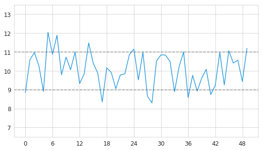
As we see, this time series exhibits a certain amount of random fluctuations, and yet its values remain close to its mean. A special case of stationary time series with mean value of zero is also called “white noise”.
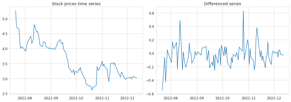
The time series can be made stationary by applying differencing, if needed - several times. Removing a fitted trend or a seasonal component (via seasonal differencing) may also be a good option. If the non-stationarity is caused by the varying variance then taking the log may also help to stabilize it. Below is an example of a stock prices time series which was hopefully made stationary by taking the first order difference.
It is possible to apply various statistical tests on the time series in order to determine whether it is stationary or not.
Needless to say that after making predictions upon such transformed stationary time series all transformations need to be reversed in order to get the final predicted value of the original series. Back to top ↑
AR models
Autoregressive (AR) models are built on the assumption that a certain value of a time series depends on its previous values. This dependence is expressed in the form of a linear regression over a certain number of the lagged values.
\[y_t = \sum_{i=1}^{p}\varphi_{i}y_{t-i}+\varepsilon_{t}\]where $\varphi$ is a set of parameters for each of the lagged values, and $p$ is the total number of lagged values.
An autoregressive process may conventionally be marked as AR(1) or AR(2), where the number at the abbreviation means the number of lags taken into account. Let’s take a look at the examples of AR processes where different numbers of lags are included, and where the coefficients have different values.
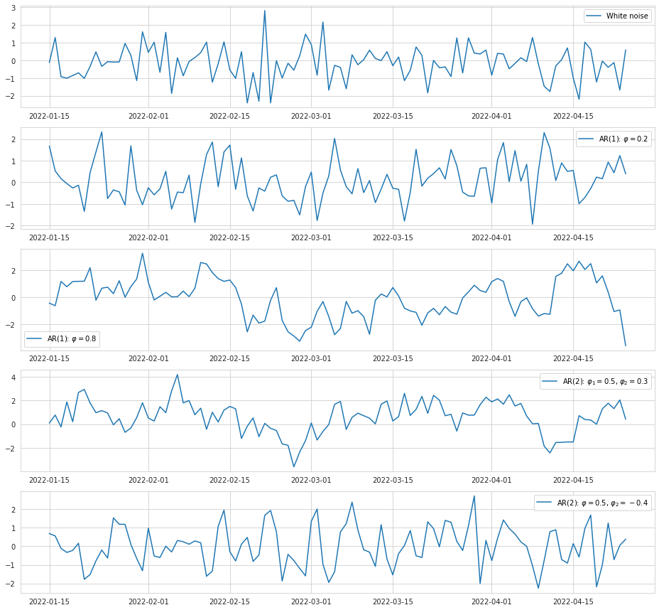
As we can see, inclusion of a single lag with a relatively low coefficient into the AR model does not make the output much different from the white noise, and the series look only slightly smoothed out. Increasing the coefficient however makes it smoother, and the series doesn’t jump around chaotically. If we include two positive terms into the model, the line starts to look more jagged compared to a single term because one additional observation from the past makes its own contribution to the next value, so that it is less impacted by its immediate predecessor. If we include two terms into the model where one is positive and another is negative, the series starts to oscillate around the mean because the negative term signifies the change in the direction. Back to top ↑
Unit root
Although AR models are built to be stationary, that is not always the case with the underlying process because it may have the unit root. The unit root is a special case of autoregression which can be expressed like this:
\[y_t = y_{t-1} + \varepsilon_{t}\]The coefficient at the regressor is one (unit), and this type of time series is in fact non-stationary. According to this model, after a disturbance in the series, the new observations no longer attempt to return to the mean value, and simply continue aimless movement from their previous position. This type of process is also known as random walk.
There are extensions of the unit root process where it may have a drift and a deterministic trend:
\[y_t = \alpha + \beta t + y_{t-1} + \varepsilon_{t}\]Below is an example of a random walk where either drift or a trend is present.
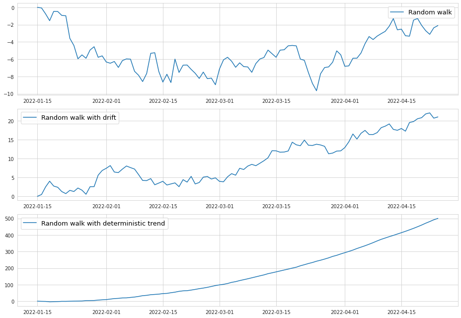
As we can see, the drift forces the time series to move generally in one direction, and it looks like a linear trend. The deterministic trend however forms an exponential pattern.
With that being said, the time series is certainly non-stationary if it has unit root. At the same time, the AR(1) process with a high positive coefficient (but less than 1) may also look like the random walk, as we saw on the example above where $\varphi_1$ was equal to 0.8. This suggests that the AR model can be viewed as a realization of a slightly “underdifferenced” time series.
MA models
Moving average time series models, or simply MA, rely on the assumption that the values are dependent on the previous deviations from the mean. They are expressed as a linear combination of the white noise as opposed to the AR models where we have a linear combination of the actual observed values.
\[y_t = \mu + \sum_{i=1}^{q}\theta_i \varepsilon_{t-i} + \varepsilon_t\]where $\theta$ is a set of parameters for each of the lagged values, and $q$ is the total number of lagged values.
The AR process incorporates all of the previous deviations (with decreasing weights) implicitly by relying on the past observations which are already impacted by those deviations. Similarly, the MA process can be viewed as a realization of all of the previous observations which led to the given deviations from the mean at $q$ past data points. Back to top ↑
Autocorrelation functions and plots
The strength of the linear relationship at different lags can be calculated using the autocorrelation function (ACF) which is similar to the correlation function in the linear regression.
\[\rho\left( k \right) = \frac{\sum_{t = k + 1}^{n}\left( y_{t} - \overline{y} \right)}{\sum_{t = 1}^{n}\left( y_{t} - \overline{y} \right)^{2}}\]where $k$ is the order of the lag, $n$ is the number of observations.
A related and no less important concept is the partial autocorrelation function (PACF) which shows the strength of the linear relationship at different lags after removing the impact of all other lags. For example, for the AR(2) process the value of a time series at $y_t$ is impacted by two previously observed values: $y_{t-1}$ and $y_{t-2}$. At the same time $y_{t-1}$ is impacted by its own two lags: $y_{t-2}$ and $y_{t-3}$. Since $y_{t-1}$ is influenced by $y_{t-2}$, its “pure” effect on $y_t$ is actually smaller than the autocorrelation function shows, and that is precisely what the partial autocorrelation function is supposed to display.
Using the values of the autocorrelation function it is possible to build ACF and PACF plots which are helpful for visual inspection of the relationships at different lags. Let’s see how these plots are different for AR and MA processes.
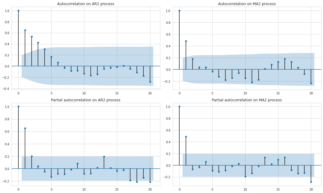
In the figure above the dark blue areas represent the confidence interval of autocorrelation not being equal to zero. In other words, only those lags whose autocorrelation goes beyond this confidence interval are considered statistically significant.
We can note that for the AR process the autocorrelation gradually declines as the number of lags increases while the partial autocorrelation drops more rapidly, and after the second lag becomes quite insignificant. This leads to a conclusion that only two lags define the AR process while all the excessive relationship seen on the ACF plot is the result of the combined effect of the lagged values.
The MA process is less dependent on the previous values because it depends only on the “innovation” part of them so we can observe that the autocorrelation plot exhibits a more rapid decline than that of the AR process, and after the second lag the correlations drop almost to zero.
In theory the ACF and PACF plots may help to understand which process we are dealing with, and how many lags to include in the model. In practice however we may not be able to inspect all of the ACF and PACF plots visually. More importantly, the data might not fit well into any of the two models, and be in fact a realization of both AR and MA which makes up the ARMA model. Back to top ↑
ARMA and ARIMA models
The ARMA model represents the time series as realization of both AR and MA processes:
\[y_t = c + \sum_{i=1}^{p}\varphi_{i}y_{t-i} + \sum_{i=1}^{q}\theta_i \varepsilon_{t-i} + \varepsilon_t\]where $c$ is some constant.
The notation ARMA(p, q) is used to depict the number of lags used for the autoregressive and moving average parts accordingly.
The further generalization of the ARMA model is the ARIMA (autoregressive integrated moving average) model. The difference between the two is that the ARIMA model assumes that the series may be non-stationary with respect to the mean so it may apply differencing as an initial step. Similarly to the ARMA, the ARIMA has its own notation of a form ARIMA$(p, d, q)$ where $d$ stands for the order of differencing.
The number of the lags which are eventually included for both autoregressive and moving average parts should be determined using grid-search and cross-validation by maximizing the likelihood of the model, or by minimizing the Akaike information criterion if the number of observations is small.
In some texts the model may be represented with the lag operator $L$, so that $y_{t - 1} = L y_{t}$. The power of $L$ represents repeated operation, so for instance $y_{t - 1}$ would be $L^{2} y_{t}$. The final ARIMA model then looks like this:
\[\begin{equation} \begin{array}{c c c c} (1-\varphi_1L - \cdots - \varphi_p L^p) & (1-L)^d y_{t} & = & c + (1 + \theta_1 L + \cdots + \theta_q L^q)\varepsilon_t\\ {\uparrow} & {\uparrow} & &{\uparrow}\\ \text{AR($p$)} & \text{$d$ differences} & & \text{MA($q$)}\\ \end{array} \end{equation}\]Or a more generic expression:
\[\varphi_p (L) \Delta^d y_t = A(t) + \theta_q (L) \varepsilon_t\]where $A(t)$ is a trend polynomial which includes the constant.
SARIMA
SARIMA is the extension of the ARIMA model which includes the seasonal terms $P$, $D$, $Q$ in addition to their non-seasonal counterparts $p$, $d$, $q$. The full model specification is this: ARIMA$(p, d, q)(P, D, Q)_{s}$, where $s$ indicates the number of observations which form the full cycle (for example 12 for monthly data).
$D$ should be understood as the seasonal differencing order, while $P$ and $Q$ are the orders of the seasonal autoregressive process and moving average respectively.
The generic form of the SARIMA model is this:
\[\varphi_p (L) \tilde \varphi_P (L^s) \Delta^d \Delta_s^D y_t = A(t) + \theta_q (L) \tilde \theta_Q (L^s) \varepsilon_t\]SARIMAX
This is yet another extension of the ARIMA model which allows in addition to the seasonal factors to also include exogenous variables. Actually, the model becomes a linear regression with residuals following the SARIMA process.
\[y_t = \beta_t x_t + u_t\]where $u_t$ is the residual which is modeled with SARIMA:
\[\varphi_p (L) \tilde \varphi_P (L^s) \Delta^d \Delta_s^D u_t = A(t) + \theta_q (L) \tilde \theta_Q (L^s) \varepsilon_t\]